next up previous
Next: Random Processes Up: Random Processes I Previous: Probability space

Random Variables

CDF:
$Prob(X(w)\le x)=F_X(x)=P(X\le x)$
props
1.
$0\le F_X(x)\le 1$
2.
FX(x) is non decreasing
3.
$\lim_{x\rightarrow -\infty} F_X(x)=0\quad \lim_{x\rightarrow \infty} F_X(x)=1$
4.
FX(x) is continuous from right

\begin{displaymath}\lim_{\epsilon\rightarrow 0} F_X(x+\epsilon)=F_X(x)\end{displaymath}

5.
$P(a<X\le b)=F_X(b)-F_X(a)$
6.
P(X=a)=FX(a)-FX(a-)

pdf:

7.
$f_X(x)=\frac{d F_X(x)}{dx}$ , if discrete we get impulses props

(a)
$f_X(x)\ge 0$
(b)
$\int_{-\infty}^{\infty} f_X(x)dx=1$
(c)
$\int_{a^+}^{b^+}f_X(x)dx=P(a<X\le b)$
(d)
$P(X\in A)=\int_A f_X(x)dx$
(e)
$F_X(x)=\int_{-\infty}^{x^+} f_X(x)dx$

Useful RV distributions

1.
Bernoulli: biasd coin flip
p - prob of success
1-p - prob of failure

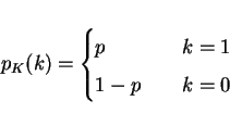
\begin{displaymath}p_K(k)=\left\{\begin{array}{ll}
\displaystyle {p} & {\qquad k=1} \\
\displaystyle {1-p} & {\qquad k=0}
\end{array}\right.\end{displaymath}

2.
Binomial (a sequence of N indept Bernoulli trials)

\begin{displaymath}P_K(k)={N \choose k} p^k(1-p)^{N-k}\qquad 0\le k \le N\end{displaymath}

3.
uniform
4.
Gaussian

\begin{displaymath}f_X(x)=\frac{1}{\sqrt{2\pi\sigma^2}}e^{-(x-m_X)^2/2\sigma^2}\end{displaymath}

5.
Poisson

\begin{displaymath}P_K(k)=\frac{(\lambda T)^k}{k!}e^{-\lambda T}\quad k=0,1,...\end{displaymath}

6.
Exponential

\begin{displaymath}f_X(x)=\lambda e^{-\lambda x} \quad x\ge 0\end{displaymath}

Functions of RV
no time to review here
But y=g(x) and fX(x) known,
first find $F_Y(y)=\int_{g(x)\le y} f_X(x)dx$
then differentiate
THIS ALWAYS WORKS! (book method doesn't always work)

More Defs

\begin{displaymath}E(X)=\int_{-\infty}^{\infty} xf_X(x)dx\end{displaymath}


\begin{displaymath}E(g(X))=\int_{-\infty}^{\infty}g(x)f_X(x)dx\end{displaymath}

nth moment

\begin{displaymath}m^{(n)}_x=\int_{-\infty}^{\infty}x^n f_X(x)dx\end{displaymath}

nth central moment

\begin{displaymath}\sigma^{(n)}_x=\int_{-\infty}^{\infty}(x-m_X)^nf_X(x)dx\end{displaymath}

$n=2 \rightarrow$ variance $\sigma^2_x$
1.
E(cX)=cE(X)
2.
E(c)=c
3.
E(X+c)=E(X)+c
4.
$var(cX)=c^2\sigma^2_x$
5.
var(c)=0
6.
$var(X+c)=var(X)=\sigma^2_x$

Characteristic functions


\begin{displaymath}\phi_X(s)=\int_{-\infty}^{\infty}f_X(x) e^{j s x}dx\quad \mbox{look like Laplace}\end{displaymath}

props

1.

\begin{displaymath}m_X^n=\left.\frac{1}{j^n}\frac{d^n \phi_X(s)}{ds^n}\right\vert _{s=0}\end{displaymath}

2.
$X~ N(m_X, \sigma)$ Gaussian

\begin{displaymath}\phi_X(s)=e^{js m_X-\frac{s^2\sigma^2}{2}}\end{displaymath}

More than 1 RV, some basic idea

\begin{displaymath}F_{X,Y}(x,y)=P(X\le x, Y\le y)\end{displaymath}


\begin{displaymath}f_{X,Y}(x,y)=\frac{\partial}{\partial x \partial y}F_{X,Y}(x,y)\end{displaymath}

Look at props (top p.155)

Covariance

E((x-mX)(y-my))=cov(X,Y)

correlation coefficient

\begin{displaymath}\rho=\frac{cov(X,Y)}{\sigma_X \sigma_Y}\end{displaymath}

Turns out that $-1\le\rho\le1$ so its a nice measure of how correlated X+Y are.
no corr.        $\rho=0$ (not indept. necessarily!!!)
same RV         $\rho=1$ (only if Gaussian)
liar         $\rho=-1$

prop

1.

\begin{displaymath}E(\sum_ic_iX_i)=\sum_i c_iE(X_i)\end{displaymath}

2.

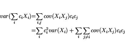
\begin{eqnarray*}var(\sum_i c_i X_i)&=&\sum_{i,j}cov(X_i X_j)c_i c_j\\
&=&\sum_i c_i^2 var(X_i)+\sum_i\sum_{j\ne i} cov(X_iX_j)c_i c_j
\end{eqnarray*}


Jointly Gaussian
2 vars


\begin{displaymath}f_{X,Y}(x,y)=\frac{1}{\sqrt{(2\pi)^2\sigma_X^2\sigma_Y^2(1-\r...
...gma_Y^2}-\frac{2\rho (x-m_X)(y-m_y)}{\sigma_X\sigma_Y}\right)}
\end{displaymath}

general


\begin{displaymath}f_X(x)=\frac{1}{\sqrt{(2\pi)^2\vert C\vert}} e^{-\frac{1}{2}(...
...ine{x}-\underline{m_X})^TC^{-1}(\underline{x}-\underline{m_X})}\end{displaymath}

where

x=[x1 x2 ... xn]T

C = cov matrix, |C|=det(C)

Props (Important since will mostly use gaussians)

1.
any subset of jointly gaussian RV's is gaussian as well
2.
completely characterized by their first and second moments
3.
conditioning still makes them jointly gaussian
i.e. fX1,X2|X3,X4 is jointly gaussian
4.
$\sum a_i X_i$ is gaussian. set of linear combos is gaussian
5.
uncorrelated jointly gaussian RV's are INDEPENDENT

RV sums

1.
Indept. RV's X+Y w/ fX(x), fY(y)

\begin{displaymath}Z=X+Y\rightarrow f_Z(z)=f_X(x)\ast f_Y(y)\end{displaymath}

Prove it!
2.
weak law of large numbers, X1,X2,... uncorrelated each w/ mean mX and $\sigma_X^2 < \infty$ then

\begin{displaymath}\epsilon>0, \lim_{n\rightarrow\infty} Prob\left[\left\vert\frac{1}{n}\sum_{i=1}^n X_i -m_X \right\vert > \epsilon \right]=0 \end{displaymath}

The empirical average converges in probability to the mean

3.
Central limit thm. X1,...,Xn indept. w/ means ( m1,...,mn) and ( $\sigma_1^2,...,\sigma_n^2$)

\begin{displaymath}Y=\frac{1}{\sqrt{n}}\sum_{i=1}^n\frac{X_i-m_i}{\sigma_i}\qquad n\rightarrow\infty\Rightarrow f_Y(y)=N(0,1)\end{displaymath}

IID? $\rightarrow Z=\frac{1}{N}\sum_{i=1}^n X_i\Rightarrow f_Z(z)=N(m_X,\sigma_x^2/n)$ when $n\rightarrow\infty$
i.e. Large sums approach a gaussian!
Very useful since physical world is often a superposition of uncorrelated events!


next up previous
Next: Random Processes Up: Random Processes I Previous: Probability space

1999-02-06